Data input in Excel
- Dec. 27, 2022
| Example files with this article: | |
Here's a new blog article after a while. Merry Christmas to all of you!
Introduction
Without any doubt there will be data entry In Excel, sometimes more, sometimes less. This goes along with time-consuming manual actions, and the risk of errors such as typos. What are our options and how do we organize best data input in Excel ? Below I will showcase a number of options, from traditional to the newest Excel functions/functionalities.
The idea is the following: for (part of) the data input we need to either select from a list, we either need to allow data input. Our case is as follows. Our data input person makes observations of birds in nature and keeps track of the species by date and name:
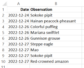
If you deal with a lot of observations on endangered birds, this duty is tedious, labourious and error-prone. Even more if it's the data input for the whole team. Luckily we have lists to pick species from (Wikipedia list):

You can then use that list in Excel to select names and speed up the work. You will copy the list to Excel, clean up a little and apply data validation. First off, you should select all 10.976 cells/bird species and give the range a name like "bird_species". Next you will apply that name in the data validation:


Did you know this option ? Even without data validation lists you can select from other input values, provided that input happened in the same column and that there are no blank cells/rows:

You will be presented a dropdown list with only the entries you already entered. The shortcut combination is Alt + arrow down, which is actually a good match; the list is expanding downwards and this is embodied by the downward pointing arrow. Note that Excel will not offer the column header "Observation" in the list: clever ! Note also that the list is sorted alphabetically: useful too.

Alt + arrow down also works fine when there are empty rows (which I discourage !) if and only if data validation as defined in that cell. In the latter case, the data validation list will be shown, instead of the "unique values from the surrounding rows in the same column".
On a personal note, I have never been a fan of those dropdown lists. Oftentimes, your hands will instinctively reach out to the mouse to make a selection frmo the list (except with Alt + arrow down) but still. This manoeuvre slows down your work with larger amounts of data input.
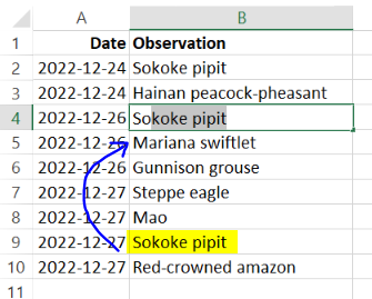
As a result I am inclined to just type names, Excel will helpfully complete the cell contents if it can recognize what I typed - if it appeared earlier in the table. In cell B4 I simply enter so and Excel completes the entry for me. I have the choice to confirm or continue typing if I don't want to use the Sokoke pipit:
A trick
Put differently, if you just want to enter the first few characters and have Excel complete it, then you can do the following. You add about 11,000 rows above the table and you copy/paste all bird species names:
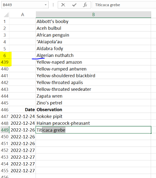
Like this, data input is quick and easy as all input has been encountered before (same column in the table). Agreed, we are cheating a bit but the end justifies the means! You can surely hide those helper cells and no one will notice. Very important: make sure that you have no empty cells/rows in between the list of names and your input table. Otherwise the completing mechanism will stop.
Attention, this autocomplete mechanism is limited to about 1,000 rows. For the really long lists, this will not provide an adequate solution. In addition, when the input is done in a data table (ListObject) the autocomplete in the table does not pick up the entries above the table. That's a pity !
To be honest, I haven't said something new until here. This trick is known in the Excel community. What if there would be empty cells? Just fill them up with a single quote and a space:
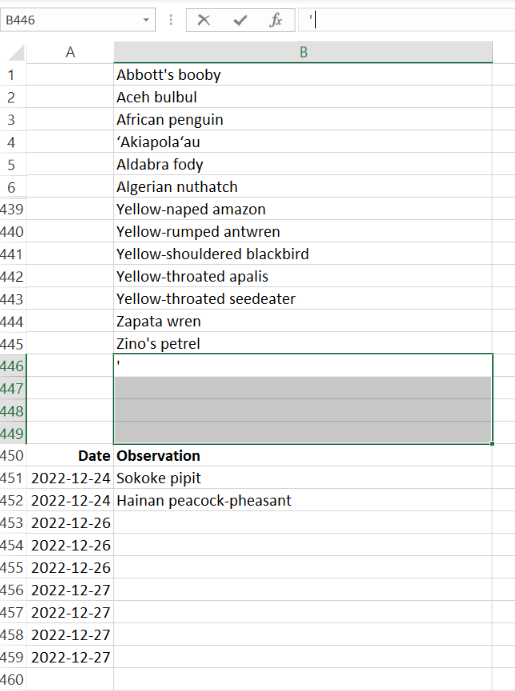
And look, you have again a contiguous range of cells! One step further. Excel MVP Randy Austin discovered this mechanism: the cells B447:B449 are effectively empty but there is a continuous trace of non-empty cells in the direction of the input table. Apparently, this is sufficient for Excel to make the connection! It's a bizarre phenomenon but it works.

Other input - new techniques
Now it's time to add new techniques for the benefit of the community, because we already knew the above. Imagine that the list of bird species would not exist but anyhow you would like to reuse your earlier inputs to facilitate new input. The earlier input exists under this form: not in a simple list but as delimited values by date. Can we get away with this format? YES!

Nowadays you can in Excel (and it's all rather new functionality):
- use dynamische array formulas
- split cell contents on character(s).
- use variables in formulas.
- use Lambda functies.
- extend or shrink ranges with a formula.
- and so on.
Here is a first formula (to build up the explanations):
=LET( data, Report!B2:B4, sep, G1, output, IFERROR( SORT( UNIQUE( TRIM( TEXTSPLIT( TEXTJOIN( sep, , data ), , sep )))), G2 ), output )
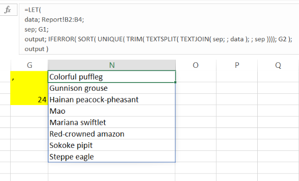
The LET function allows us to define variables. Here we deal with "data", "sep" and "output". "data" and "sep" are simple references to other cells, "output" actually calculates a result. "output" splits the contents of cells B2:B4 on the separator (", "). Next we take all unique items, without extra spacing, we sort the list and show the list as of cell N1. The result, for the current input on the other sheet, is cells N1:N8. Have a look at how the list will expand and shrink with the unique bird species in the source cells. A blue border will appear surrounding the range N1:N10 to indicate that it's dynamic array formula. The cell N1 contains the formula, the cells N2:N8 do not contain a formula but they receive the "spilled" results from the above formula. Cell G2 is empty and will be discussed in shortly. After defining 3 variables in the LET function "output" as hte last argument within the function will the the result of the formula in the cells.
Very nice! But we want to continue with the theme of this article: how to speed up data input and make it easier ? As a matter of fact, we want to extend the list of (currently) 10 different bird species in the same column with new data input. But we also know that we cannot use empty rows of the mechanism to complete cells will fail. On the other hand, we also don't want to move our input table down every once in a while since we have too many different names in the lookup list - too little space to show them.
My solution
What would you think if we were to ask Excel to extend the list for us ? To make it a bit more concrete: data input occurs as of row 25. Put differently, a header row in row 24 ensures that we can already list 23 unique bird species names. Currently we have 10, so 13 empty cells remain. Let's fill up those empty cells such that they are not empty anymore, and automatically completing text entries is possible again.

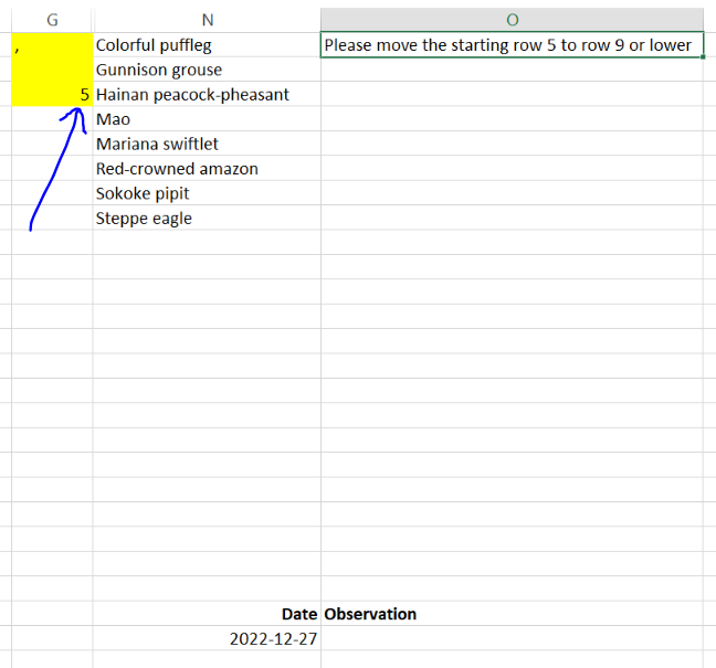
That should be visible in the picture above. The dynamic array formula extends until row 24, this is what we set in cell G3, the variable "padding_char". Choose the variable names to your own liking ! The formula will be as such:
=LET( data, Report!B2:B4, sep_char, G1, starting_row, G3, padding_char, G2, uniques, IFERROR( SORT( UNIQUE( TRIM( TEXTSPLIT( TEXTJOIN( sep_char, , data ), , sep_char )))), padding_char ), output, IF( COUNTA( uniques ) >= starting_row, "Please move the starting row " & starting_row & " to row " & COUNTA( uniques ) + 1 & " or lower", EXPAND( uniques, starting_row - 1, , padding_char )), output )
The attentive reader will understand that I take into account the situation whereby the starting_row (24) is "too high", in other words, there is too little room for the unique bird species. In this case there will be a notification in the cell, saying that the starting row should be moved downwards. The unique bird names will not be shown, instead the notification is shown to the user.
Lambda formulas
The last step, to round up this task, is een heuse Lambda function. Daarbij definiëren we een nieuwe function zodat die overal in het Excel bestand toegepast kan worden. De laatste stap in het rijtje, om het allemaal af te maken, is a new Lambda function. We will effectively define a new function that can be applied in the entire workbook. It's as if the new function existed forever in Excel. The function can accept arguments (including optional arguments) and very much resembles what we already had in the LET function:

Please have a look in the example file to understand how this is all done. Lambda functions are very versatile and do replace both VBA code and existing formulas with helper cells/columns. They can also be recursive.
Data validation list
These functions that return the unique entries (without padding) could be stored in a cell. The results will spill to the cells below. That dynamic range could be given a name, and that name could be used in a simple Data validation list. For example: =Source_Cells which refers to: =T1# Here, the hash symbol # is called the spill range operator. T1# refers to the dynamic range starting in cell T1.
Lastly, I would like to mention the FILTER function. That function allows you to create a dynamic array containing for instance, all cells matching *yellow*. That helper list could guide the user on new data entry about yellow birds.
Useful shortcuts
When it comes to data entry, I very often find myself using these shortcuts:
- Alt + arrow down: pick an item from a list
- Ctrl + D: copy the cell(s) above to the currently selected cell(s). The copy action does all cell properties. The direction is Down.
- Ctrl + ": copy the cell value above to the currently selected cell. The copy action does only transfer the cell text (formula result).
- Ctrl + R: similar to the variant with D but the direction is to the Right.
- Ctrl + Enter: select multiple cells, enter a value or formula, and then hit this shortcut to have Excel fill all selected cells at once.
