Spot duplicates in a hierarchy to avoid circular references
- Jan. 28, 2021
| Example files with this article: | |
Introduction
In IBM Planning Analytics, consolidation structures can be created within hierarchies (dimensions). They allow us to roll up and aggregate underlying data in a very efficient way. In any hierarchy, all elements should be named in a unique way, paying attention to the fact that there is case-insensitivity and also space-insensitivity. This means that we cannot distinguish 2 elements by merely adding a space or changing the case of the characters.
If we try to create / maintain hierarchical relations where errors are made against these rules, we will typically see circular references: adding an element as a child to a same-named parent, this is not allowed. Every once in a while I am confronted with this issue at the customer, generally speaking when dimensions are long and contain multiple levels. I used Excel formulas to identify the issue in Excel straight away, such that the customer can immediately see which source data records pose issues.

In the screenshot above you will find coloured cells on rows 6, 8, 10. Each of the rows has an issue:
- On row 6, columns B and C are equal for TM1 because the double space in the middle does not distinguish the account consolidation names.
- On row 8, columns B and E are equal for TM1 because the trailing space at the end of the cells will not be sufficient.
- On row 10, columns B and C are highlighted here because there is an Alt-Enter character at the end of the B10. Best is to avoid such issues because in csv format it could lead to records being chopped off.
My new formula is stored in column H. You can add conditional formatting to colour the offending account names by filtering on 'TRUE'. The orange color was applied manually by myself.
Advanced Excel formulas
Here it is:
=LET( d, A2:G2, c, CLEAN( TRIM( SUBSTITUTE( d, CHAR(160), " " ))), f, FILTER( c, c <> "" ), COUNTA( UNIQUE( TRANSPOSE( f ))) < COUNTA( f ))
Let's break it down and please have a look at the colourful arrows down below:
- The LET formula allows to use variables. I define d (data), c (cleaned), f (filtered).
- After the definition of each variable, where you can easily reference variables that were defined earlier, the last argument to the LET formula is the actual calculation: I ask Excel to filter out the (filtered) account names when the number of unique accounts names is strictly less than the number of names.
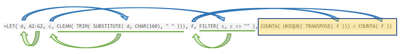
The FILTER and UNIQUE formulas are new in Excel. They are dynamic array formulas and very useful ! They can save us a lot of headaches and workarounds (even up to pivot tables or VBA). As the UNIQUE formula can also be used to evaluate ranges that span multiple columns as "1 row", we need to TRANSPOSE our "1 row/7 column" range into a "7 rows/1 column" range.
That's it! You are now free to autofilter the list (or use another FILTER function :-) ) and present it to the customer for review / adjustments.