Your favorites with formatting
- Nov. 15, 2020
| Example files with this article: | |
Favorite travel destinations
Over the last year or so the Excel product teams introduced a number of new things, a.o. dynamic arrays. It centers around looking in a different way at Excel formulas and their argumenten, for existing functions, and also that a number of new functions have been added to the software. In this article I will show you some of these new functions, as well as an example of what I mean with using existing functions in a different way. We could say that in some sense, dynamic array formulas replace existing array formulas (the ones you enter with Ctrl + Shift + Enter), and they have the benefit of shortening and simplfying ridiculously long formulas !
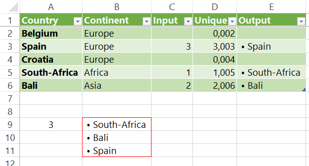
While we are all in lockdown we can dream about our favorite travel destinations… Imagine you enntered a number of these in an Excel table. By numbering countries you will indicated your preferences: 1 is the highest preference, followed by 2, 3, etc. A tie is possible too, for instance 3 times number 2. Our purpose is to automatically generate a list of the chosen travel destinations, in descending order of preference. No VBA code, no events, no PowerQuery, no manual interventions. Just Excel formulas ! And… as an extra we want the red border surrounding the list of countries: the number of rows is dynamic because it depends on how many travel destinations we single out. How can we do all this ? Let me help you and show it. First have a look at the picture and download the example file near the top of the page.

Our table starts in cell A1, it's a table in the Excel sense, a ListObject. You can see the small blue icon near the bottom right border in cell E6, the last cell of the table. Excel takes care of the formatting (the even and odd row formatting for instance) and makes sure that formulas are dragged down as far as needed.
Then you can put numbers in column C ("Input"). In principle it will be 1, 2, 3, … but if wanted you can also use other numbers. The smallest number gets the highest preference, then the second smallest, etc. Numbers can be used more than once. Column D ("Unique") takes those numbers from column C and returns only unique numbers. The formula knows how to deal with blanks in column D, just as ties. The aim is to sort on column D, using a simple formula. Let's first have a look at column E ("Output"): there we have a bullet point in front of the country name. I did not use cell formatting but rather a character that represents such a bullet point. Below in the article I will present an overview of the formulas I used.
So the table should be clear by now. Let's jump to the complex formula in cell B9 for the list of chosen destinations:

The formula is complex but inside out we can dismantle it:
- Tbl_Country[Unique]: the like-named column in the table (that I called "Tbl_Country")
- Tbl_Country[Input]: the like-named column in the table
- FILTER( Tbl_Country[Unique]; Tbl_Country[Input] > 0 ): return all values from the column "Unique" where the column "Input" is greater than 0 - each time for the same row
- SORT( PREVIOUS LIST ): we are going to sort that list, ascending smallest to greatest
- VLOOKUP( PREVIOUS SORTED LIST; Tbl_Country[[Unique]:[Output]], 2, 0 ): now we are going to do a lookup of each of the (3) numbers in the column "Unique" and a VLOOKUP() gets the results from the "Output" column ("Output" is the 2nd column from the range Tbl_Country[[Uniek]:[Output]])
You don't need to type all the names of columns and tables: you can select them using the mouse and Excel will complete the formula. We have a much easier formula in cell A9: we notice the number of items in the returned list to the right of it. The syntax is probably new to many of the readers: it's the # symbol. This symbol turns cell B9 into the "spill range" B9. At this moment the spill range is B9:B11, because the gigantic formula returns values in the range B9:B11. It could be different tomorrow, when we have more or fewer favorite travel destinations.
This is very important: leave some space below the "spill range" because it could be that you select more countries in the future. As such, Excel will need more space to return the output.
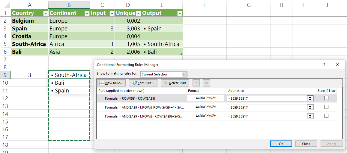
A dynamic border

We can solve this with the ROW() function. Have a detailed look in the attached file, it isn't very difficult. The only difficult thing is that we need 3 different rules for the conditional formatting. This could have been easier Microsoft, but I digress.
Summary
In this article we saw that a number of new functions were added to Excel, besides FILTER() and SORT() there are a few others. We will discuss them in a follow up article. Next to that we applied the VLOOKUP() formula (an existing one) to a dynamic range, and therefore that VLOOKUP() will not only return 1 value but a dynamic number of values. Finally we added formatting to a dynamic range, also here without any VBA code and using only built-in Excel functionalities. One of the benefits is that we don't need to filter and sort manually, or work with hidden rows, etc.
